Value-Function Approximation

So far we represented value functions using lookup tables where each state \(s\) has an entry \(V(s)\), or every state-action pair \(s,a\) has an entry \(Q(s,a)\). The problem with this is that in most real world scenarios there are too many states and/or actions to store in memory, and it's too slow to learn the value of each state individually.

In a very large state/action-space, if we learn the value of some state \(s=9\), but never visit \(s=10\), then knowing something about state 9 gives us no help when we are in state 10, that is to say, we have no generalization.

To solve this we can estimate value functions using function approximation: \[\hat{v}(s,w) \approx v_{\pi}(s)\] \[\hat{q}(s,a,w) \approx q_{\pi}(s,a)\] So we can generalize from seen states to unseen states by updating the parameter \(w\) by using MC or TD learning. For the rest of this section we'll focus on approximating the state-action function \(Q(s,a)\) because the state-value function isn't very useful for in model-free settings as we saw in [[6 Model-free Control]].

Setup

Here we describe how to do function approximation in the RL setting. We use stochastic gradient descent just like in typical deep learning, and can use any differentiable function to represent the value function, but in this case we will just use a simple linear combination. Here we also assume an oracle value function \(q_{\pi}\) as the "truth" values which are given in a supervised learning setting, but will update this assumption later.

1. Represent state using a feature vector where each feature represents something about the state \(S\) \[ \mathbf{x}(S,A) = \begin{pmatrix} \mathbf{x}_1(S,A) \\ \vdots \\ \mathbf{x}_n(S,A) \end{pmatrix} \]
2. Represent the value function by a linear combination of features, this is the function of weights that we'll try to improve \[\hat{q}(S,A,w) = \sum^{n}_{j=1} x_j(S,A)w_j\]
3. Objective function is the mean-squared error \[J(w) = \mathbb{E}_{\pi}[(q_{\pi}(S,A) - \hat{q}(S,A,w))^2]\]
   • Remember that \(q_{\pi}\) is the hypothetical oracle value function
4. Weight update = step-size x gradient, where gradient = (inner derivative x outer derivative) \[\nabla_w \hat{q}(S,w) = x(S,A)\] \[\Delta w = \alpha\underbrace{(q_{\pi}(S,A) - \hat{q}(S,A, w))}_{\text{error}}\underbrace{\nabla_w \hat{q}(S,A, w)}_{\text{gradient}}\]
5. So the weight update ends up being same as in deep learning:\[w \leftarrow w + \Delta w\]

Incremental Control Algorithms

Above was a general framework that assumed an oracle value function \(q_{\pi}\). But in RL the goal is to learn from experience not some truth values or oracle as in supervised learning, so let's update this general framework with RL.

We substitute a target for \(q_{\pi}(S,A)\): \[\Delta w = \alpha \underbrace{(\textcolor{red}{q_{\pi}(S,A)} - \hat{q}(S,A, w))}_{\text{error}} \underbrace{\nabla_w \hat{q}(S,A, w)}_{\text{gradient}}\]

• For Monte-Carlo, the target is the return \(G_t\) \[\Delta w = \alpha \underbrace{(\textcolor{red}{G_t} - \hat{q}(S,A, w))}_{\text{error}} \underbrace{\nabla_w \hat{q}(S,A, w)}_{\text{gradient}}\]
• For SARSA (TD) the target is the TD target \(R_{t+1} + \gamma Q(S_{t+1}, A_{t+1})\) \[\Delta w = \alpha \underbrace{(\textcolor{red}{R_{t+1} + \gamma \hat{q}(S_{t+1}, A_{t+1})} - \hat{q}(S,A, w))}_{\text{error}} \underbrace{\nabla_w \hat{q}(S,A, w)}_{\text{gradient}}\]
• For forward-view TD(\(\lambda\)) the target is the action-value \(\lambda\)-return \[\Delta w = \alpha \underbrace{(\textcolor{red}{q_t^{\lambda}} - \hat{q}(S,A, w))}_{\text{error}} \underbrace{\nabla_w \hat{q}(S,A, w)}_{\text{gradient}}\]
• For backward-view TD(\(\lambda\)), the equivalent update is \[ \begin{align} \delta_t &= R_{t+1} + \gamma \hat{q}(S_{t+1}, A_{t+1}, w) - \hat{q}(S_t, A_t, w) \\ E_t &= \gamma \lambda E_{t-1} + \nabla_w \hat{q}(S_t, A_t, w) \\ \Delta w &= \alpha \underbrace{\delta_t}_{\text{error}} \underbrace{E_t}_{\text{trace}} \end{align} \] Note that in the TD methods we used \(\hat{q}(S_{t+1}, A_{t+1}, w)\), which is the approximated value function's guess for the state-action value of \((S_{t+1}, A_{t+1})\).

Batch Reinforcement Learning

The issue with online incremental learning is that it only uses each sample once and doesn't fully exploit available data. The problems with this are:

1. Neural networks learn incrementally, you usually need multiple passes through the data to get optimal parameters
2. In RL, targets keep changing since the value functions themselves are estimates that improve as we learn. Early in training our value estimates are poor so we need multiple passes as these targets get better. e.g. the value of state A would be inaccurate at first pass, but much more accurate on later passes
3. In sequential experience the state \(S_{t+1}\) is highly correlated with \(S_t\). Training a neural network on such correlated data is inefficient and can lead to unstable learning

Experience Replay

In experience replay, we learn an action-value function by training on errors from a dataset of experience that we collected from a prior policy.

Here's the process:

1. Initialize Replay Memory: Create a large buffer or memory, \(D\), which can hold a vast number of experience tuples.
2. Gather Experience: As the agent interacts with the environment using some exploration policy (e.g., \(\epsilon\)-greedy), we store the transition tuple \((S_t, A_t, R_{t+1}, S_{t+1})\) in the replay memory \(D\).
3. Learn from mini-batches: At each training step, instead of using the most recent experience, we sample a random mini-batch of transitions \((S_j, A_j, R_{j+1}, S_{j+1})\) from \(D\).
4. Calculate the Target and Update: For each transition in the mini-batch, we calculate the Q-learning target. This is an off-policy update, as we are learning the value of the greedy policy while we may have been following an exploratory policy to gather data. The target is: \[y_j = R_{j+1} + \gamma \max_{a'} \hat{q}(S_{j+1}, a', w)\]
5. We then perform a gradient descent update on the weights \(w\) using the mean squared error between our network's prediction \(\hat{q}(S_j, A_j, w)\) and the target \(y_j\):\[\Delta w =\alpha (y_j - \hat{q}(S_j, A_j, w)) \nabla_w \hat{q}(S_j, A_j, w)\]

Deep Q-Networks (DQN)

DQN uses experience replay and fixed Q-targets. Regular Q-learning with function approximation has a moving target problem. In the loss function, both the target and prediction depend on the same weights \(w\): \[L(w) = \mathbb{E}\left[\left(r + \gamma \max_{a'} \hat{q}(s', a'; \mathbf{w}) - \hat{q}(s, a; \mathbf{w})\right)^2\right]\]

This creates instability because:

• You update \(w\) to make \(\hat{q}(s,a;w)\) closer to the target
• But the target \(r + \gamma \max_{a'} \hat{q}(s', a'; w)\) also changes since it uses the same \(w\)
• It's like chasing a target that moves every time you move toward it!

This leads to oscillating Q-values, unstable training, and poor convergence.

Fixed Target

DQN uses two sets of weights:

• Current weights \(w\): used for predictions \(\hat{q}(s, a; w)\) - these get updated every step
• Fixed weights \(w^-\): used for targets \(r + \gamma \max_{a'} \hat{q}(s', a'; w^-)\), these stay frozen

The DQN loss becomes: \[L_i(w_i) = \mathbb{E}\left[\left(r + \gamma \max_{a'} \hat{q}(s', a'; \mathbf{w_i^-}) - \hat{q}(s, a; \mathbf{w_i})\right)^2\right]\] The fixed weights \(w^-\) are periodically updated (e.g., every 1000 steps) by copying: \(w^- \leftarrow w\). So now we have:

• Stable targets: Target doesn't change during a batch of updates
• Consistent learning direction: Multiple gradient steps toward the same target
• Better convergence: No more moving target chaos

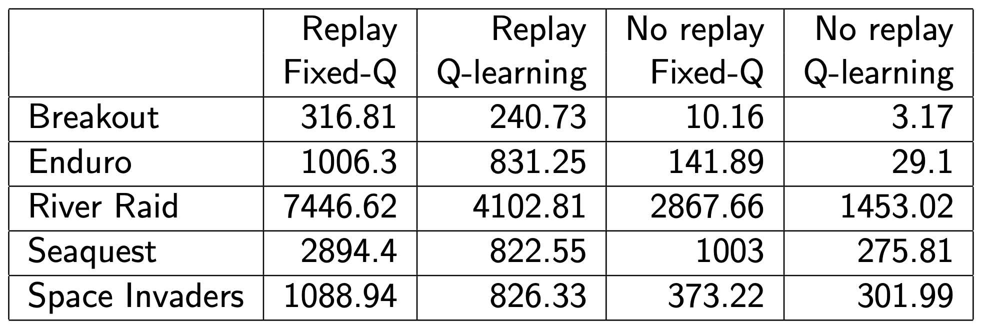
The following table shows how important fixed targets are in practice: