Policy and Value Iteration

Preface

This note is the first in a series of notes covering the basics of Reinforcement Learning (RL), my goal in this series is to not just explain the material, but try to make it intuitive with detail, or visual example, in areas where I found myself lacking explanation when I was learning it. Most of this material comes from David Silver's RL course (which I believe is still the best out there for the basics), including the images dispersed throughout. I will assume knowledge of Markov Decision Processes and Dynamic Programming as prerequisites.

Introduction

Our end goal in RL is to find an optimal policy \(\pi^*(a|s)\) that solves the decision making problem. A useful tool in doing that is finding the optimal value-function \(v^{*}(s)\) because we can use it to go to the most valuable state next.

The prediction problem in RL is to estimate value functions \(v_{\pi}\) or \(q_{\pi}\) that tell us how good difference states or state-action pairs are under a given policy. The control problem in RL is to find an optimal policy \(\pi^*\) that maximizes expected return (gets us to our goal optimally).

It's important to note that the prediction problem is a subproblem of the control problem. In order to find the optimal policy, we need to know what the value function(s) are so we can build a policy by knowing which state/action to pick.

Policy Evaluation

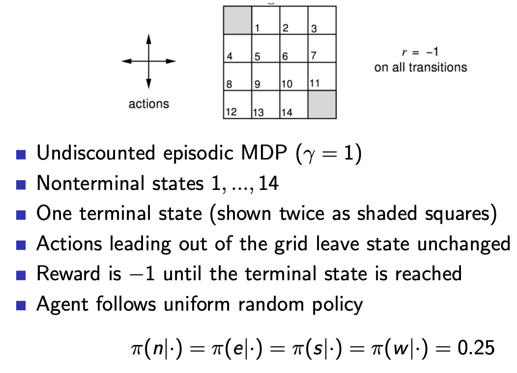
We can use policy evaluation to evaluate a policy \(\pi\) and find the state value function \(v_{\pi}\) following that policy. Policy evaluation is essentially an iterative application of the Bellman equation for state values under a fixed policy.

The Bellman equation for state values under policy \(\pi\) is given: \[v_{\pi}(s) = \mathbb{E}\left[R_{t+1} + \gamma R_{t+2} + ... | S_t = s\right]\] \[v_{\pi}(s) = \sum_{a}\pi(a|s)\left[R(s,a) + \gamma \sum_{s'}p(s,a,s') v_{\pi}(s')\right]\] And the policy evaluation algorithm applies the following \(\forall s \in \mathcal{S}\): \[v_{k+1}(s) = \sum_{a}\pi(a|s)\left[R(s,a) + \gamma \sum_{s'}p(s,a,s') v_{k}(s')\right]\]

Example

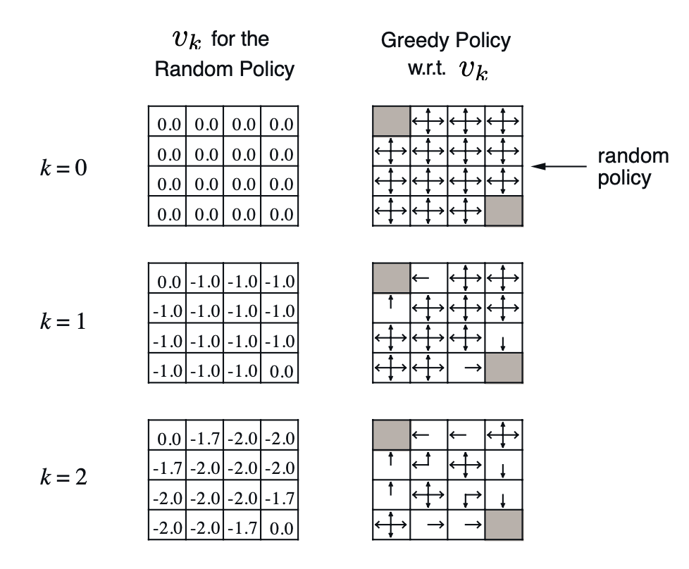
We can see in the following example that each step updates the value function closer to \(v_{\pi}\). In the particular case of state 1 between k=1 and k=2, the update goes as follows: \[v_2(1) = 0.25 × [-1 + (-1.0)] + 0.25 × [-1 + (-1.0)] + 0.25 × [-1 + (-1.0)] + 0.25 × [-1 + 0.0] = -1.75\]

Policy Iteration

We use policy iteration to improve a policy \(\pi\) towards the optimal policy \(\pi^*\). The algorithm goes as follows:

Loop:

1. Policy evaluation Estimate \(v_{\pi}\) using iterative policy evaluation (above) \[v_{\pi}(s) = \mathbb{E}\left[R_{t+1} + \gamma R_{t+2} + ... | S_t = s\right]\]
2. Policy improvement Generate \(\pi' \geq \pi\) using greedy policy improvement \[\pi' = \text{greedy}(v_{\pi})\]\[\pi^*(s) = \text{argmax}_a q^*(s,a)\] The greedy policy improvement step works because if we act greedily with respect to \(v_{\pi}\) in any state, we get a policy that is at least as good as \(\pi\). The algorithm stops when \(\pi' = \pi\) (no policy change, or very little change) which happens iff \(\pi\) satisfies the Bellman optimality equation \[v_{\pi}(s) = \text{max}_{a} q_{\pi}(s,a)\] Note that argmax returns the value of the provided argument that maximizes the function, and max returns the largest output of the function by the provided argument.

Value Iteration

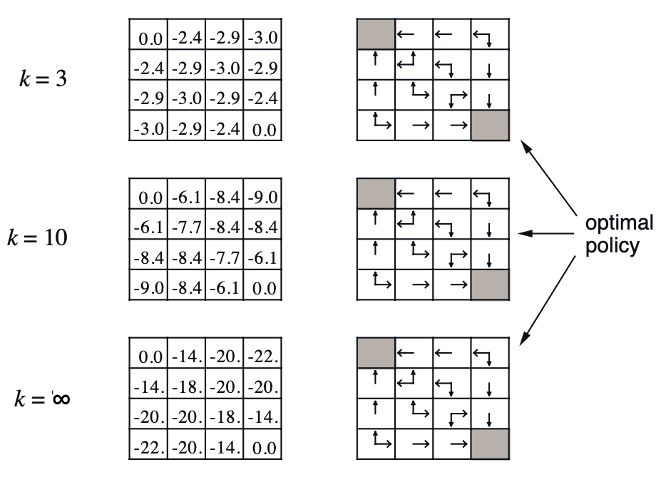
The drawback with policy iteration sometimes is that it evaluates policies to full convergence of the value function, even if that policy is not a good one, wasting a lot of time. In the policy evaluation example above the greedy policy does not change after k=3, but the policy evaluation continues for much longer. Value iteration does not have that problem.

For value iteration, we use the Bellman optimality equation, the key part being the addition of the max: \(v_{k+1}(s) = \text{max}_a \left[R(s,a) + \gamma \sum_{s'} P(s'|s,a) V_k(s')\right]\)

Again we allow the value function to converge (minimal change step over step), and then extract the final greedy policy \[\pi(s) = \text{argmax}_a \left[R(s,a) + \gamma \sum_{s'} P(s'|s,a) V(s')\right]\]

Example

Applying the value iteration to our example from above we get the following iterations:

For example, calculating \(V_2(4,2)\) using the \(V_1\) values: Calculate value for each action:

• Right: \(-1 + 1 \times V_1(4,3) = -1 + 1 \times (-1) = -2\)
• Left: \(-1 + 1 \times V_1(4,1) = -1 + 1 \times (-1) = -2\)
• Up: \(-1 + 1 \times V_1(3,2) = -1 + 1 \times (-1) = -2\)
• Down: \(-1 + 1 \times V_1(4,2) = -1 + 1 \times (-1) = -2\)

\(V_2(4,2) = \max\{-2, -2, -2, -2\} = -2\)

k = 0 (Initial values): \[\begin{bmatrix} 0.0 & 0.0 & 0.0 & 0.0 \\ 0.0 & 0.0 & 0.0 & 0.0 \\ 0.0 & 0.0 & 0.0 & 0.0 \\ 0.0 & 0.0 & 0.0 & 0.0 \end{bmatrix}\] k = 1: \[\begin{bmatrix} 0.0 & -1.0 & -1.0 & -1.0 \\ -1.0 & -1.0 & -1.0 & -1.0 \\ -1.0 & -1.0 & -1.0 & -1.0 \\ -1.0 & -1.0 & -1.0 & 0.0 \end{bmatrix}\]

k = 2: \[\begin{bmatrix} 0.0 & -1.0 & -2.0 & -2.0 \\ -1.0 & -2.0 & -2.0 & -2.0 \\ -2.0 & -2.0 & -2.0 & -1.0 \\ -2.0 & -2.0 & -1.0 & 0.0 \end{bmatrix}\] As you can see, value iteration will converge much sooner than policy iteration here.

Difference between PI and VI

Value Iteration simultaneously finds the value of each state and the best policy by iteratively choosing the best action at each state, then extracts the final greedy policy from the converged value function.

Policy Iteration alternates between two phases: fully evaluating the current policy to find state values, then improving the policy by acting greedily on those values, repeating until the policy stops changing.

Sometimes textbooks try to show the equivalence between policy and value iteration by re-writing value iteration as follows:

Step 1: \(\pi(s) = \text{argmax}_a \sum_{s'} p(s'|s,a)[r(s,a,s') + \gamma v(s')]\) (policy improvement)
Step 2: \(v(s) \leftarrow \sum_{s'} p(s'|s,\pi(s))[r(s,\pi(s),s') + \gamma v(s')]\) (one policy evaluation step)

How New Information Emerges

Both algorithms work by propagating reward information backward from terminal states:

• Iteration 1: States one step from terminal rewards learn their true expected values
• Iteration 2: States two steps away incorporate information from iteration 1 states
• Iteration k: Information has propagated k steps backward from terminal states This creates a "ripple effect" where accurate value information spreads outward from reward sources through the state space.

In Value Iteration: Information propagates one step per iteration across all states simultaneously In Policy Iteration: During policy evaluation, information propagates to convergence for the current policy, then the improved policy shifts which paths the information flows along

The discount factor \(\gamma\) controls how this information attenuates as it travels, distant states receive proportionally smaller updates, which naturally captures the decreasing influence of far-future rewards.