Model-free Prediction

In model-free settings we no longer assume complete knowledge of the environment, that is, the reward function \(R(s,a)\) and the transition probabilities \(P(s,a,'s)\) are no longer known. To find optimal policies we must now learn from experience. This more closely resembles real-world examples because we rarely have full knowledge of the environment.

For now we will discuss model-free prediction, so as a reminder, the prediction problem, a subproblem of the control problem, is to estimate state and action value functions \(v_{\pi}\) and \(q_{\pi}\) that tell us the value of a state and state action pair respectively.

Monte-Carlo Learning

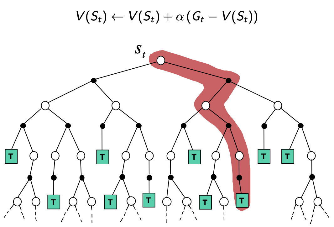
Monte-Carlo methods learn from experience, by sampling or generating episodes of experience, and computing the empirical mean return instead of the expected return.

Monte-Carlo Policy Evaluation

Goal: learn \(v_{\pi}\) from episodes of experience under policy \(\pi\) \[S_1, A_1, R_2, \ldots S_k \sim \pi\] First-Visit Monte-Carlo Policy Evaluation To evaluate state \(s\), the first time-step \(t\) that state \(s\) is visited in an episode:

1. Increment counter \(N(s)\leftarrow N(s) + 1\)
2. Increment total return \(S(s) \leftarrow S(s) + G_t\)
3. Value is estimated by mean return \(V(s) = \frac{S(s)}{N(s)}\) By the law of large numbers, \(V(s) \rightarrow v_{\pi}(s)\) as \(N(s) \rightarrow \infty\)

Note that we know \(G_t\) because we can sum the rewards for all future actions from any given state since we already have the sequence of episodes of experience.

Every-Visit Monte-Carlo Policy Evaluation Same as first-visit, except perform the actions on every visit to \(s\).

Blackjack Example

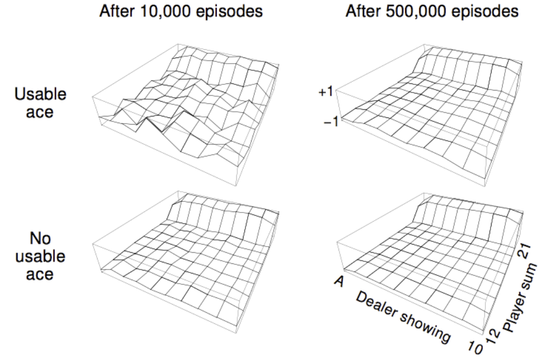
As an example, this is the value function from a Monte-Carlo policy evaluation of a blackjack policy that sticks if sum of cards \(\geq 20\), otherwise hits. Notice the value of the player having a 21, if the dealer is showing an ace is low, this is because the dealer has the chance of drawing a face card and pushing/tying. Also note that the graph for the usable ace is less smooth, this is because usable aces are rare in experience so it takes more time to learn their true value.

Incremental Monte-Carlo Updates

• To make this more "online" and remove the need to track old episodes (S(s)), we can update \(V(s)\) incrementally after each episode \(S_1, A_1, R_2, \ldots, S_T\)
• For each state \(S_t\) with return \(G_t\):
  • \(N(s)\leftarrow N(s) + 1\)
  • \(V(S_t) \leftarrow V(S_t) + \alpha(G_t - V(S_t))\)
  • Where \(\alpha\) is some kind of learning rate and the second term is the error

Temporal-Difference Learning

Temporal-Difference (TD) methods also learn directly from episodes of experience, but they can learn from incomplete episodes, by bootstrapping. They essentially update a guess towards a guess.

In incremental every-visit Monte-Carlo:

• Update value \(V(S_t)\) toward actual return \(\textcolor{red}{G_t}\)
  • \(V(S_t) \leftarrow V(S_t) + \alpha(\textcolor{red}{G_t} - V(S_t))\)

In TD(0):

• Update \(V(S_t)\) toward estimated return \(\textcolor{red}{R_{t+1} + \gamma V(S_{t+1})}\), so the update becomes:
  • \(V_{new}(S_t) \leftarrow V_{old}(S_t) + \alpha(\textcolor{red}{R_{t+1} + \gamma V(S_{t+1})} - V_{old}(S_t))\)
• \(R_{t+1} + \gamma V(S_{t+1})\) is called the TD target
  • \(R_{t+1}\) comes from experience and \(V(S_{t+1})\) is the model's current guess
• \(\delta_t = R_{t+1} + \gamma V(S_{t+1}) - V_{old}(S_t)\) is called the TD error

MC vs. TD

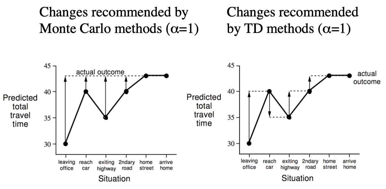
In the following example where the value at each state is predicted time remaining, we can see that Monte Carlo methods recommend that each state in the chain adjust their prediction to the actual outcome. Whereas the TD methods suggest that each state update it's value to the prediction of the next state.

Bias-Variance Tradeoff

• Bias: How far off your estimation method is from the true value on average across many episodes.
• Variance: How much your individual estimates jump around from episode to episode.

Monte-Carlo learning is unbiased because it depends on the actual return which is obviously an unbiased estimate of your true performance. But it has very high variance because it depends on \(n\) steps that could add any amount of variance to the total. In driving: depends on every traffic light, every other driver's behavior, construction, weather, etc.

TD learning on the other hand is biased because it depends on our current estimate of the value of \(V(S_{t+1})\), but it has much lower variance since it only depends on one random step. In driving: only depends on what happens between leaving office and reaching the car.

In reality we don't have much data and high variance data can be particularly damaging. So it's better to depend on stable estimates that are slightly wrong (biased but low variance) than wildly fluctuating estimates that are right on average (unbiased but high variance). You learn faster and more reliably.

Advantages of TD Learning

• Online learning TD can learn immediately from each step, while MC must wait for complete episodes, which sometimes do not occur.
• Sample efficiency TD makes better use of limited data, each step provides a learning opportunity, whereas MC only learns once per episode.
• Robustness to Outliers If a particular trip took 43 mins due to unusual traffic, MC will aggressively push all state values towards 43. TD's smaller incremental updates are less likely to be thrown off by one unusual episode.
• Faster convergence If an episode has 100 steps, TD makes 100 updates whereas MC makes 1 update.

Unified View

• Monte-Carlo learning is a one directional look-ahead to a terminal state.
• Temporal Difference learning is a one directional look-ahead to the next state.
• Dynamic programming is an all directional look-ahead to the next state.

Monte-Carlo Backup

Temporal-Difference Backup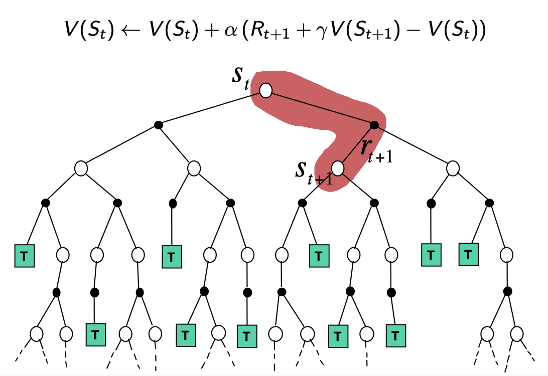

Dynamic Programming Backup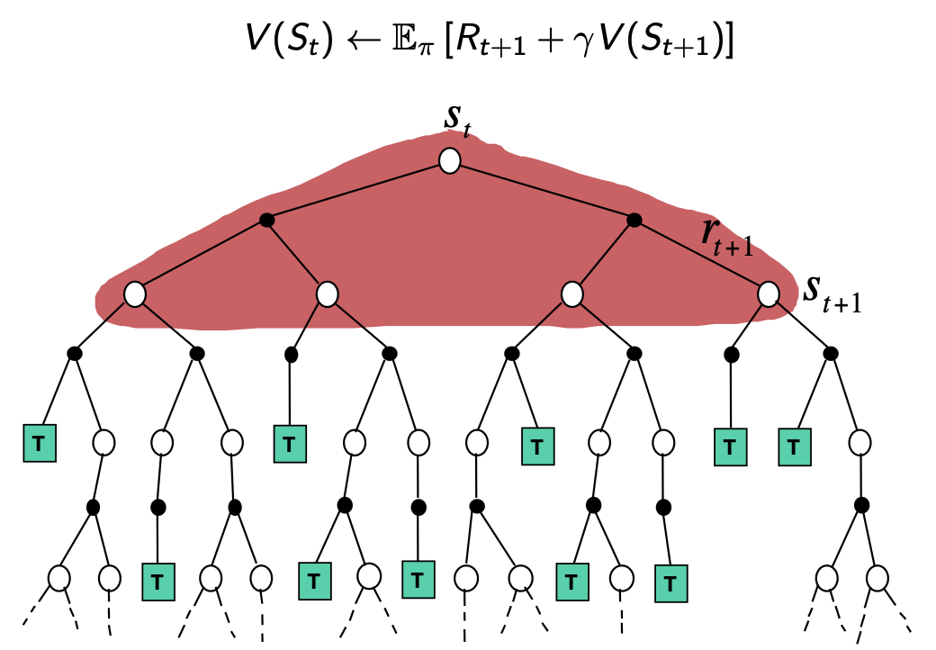

\(TD(\lambda)\)

MC and TD learning are on a spectrum on how far into the future you look to decide the state value, we could select any number \(n\) of steps forward to look. But it's difficult to know what exact number of steps to look forward for any given environment/scenario, so we develop a method to efficiently combine information from all time-steps.

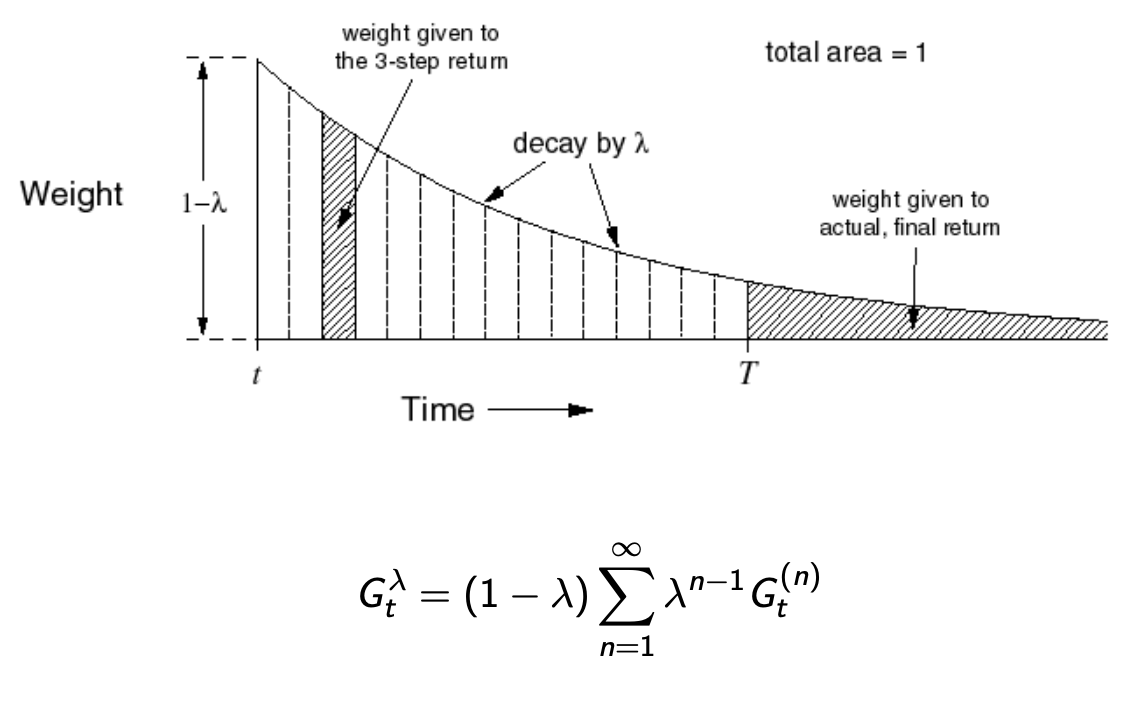
We use the \(\lambda\)-return \(G^{\lambda}_t\) that combines all \(n\)-step returns \(G^{(n)}_t\) using weight \((1-\lambda)\lambda^{n-1}\):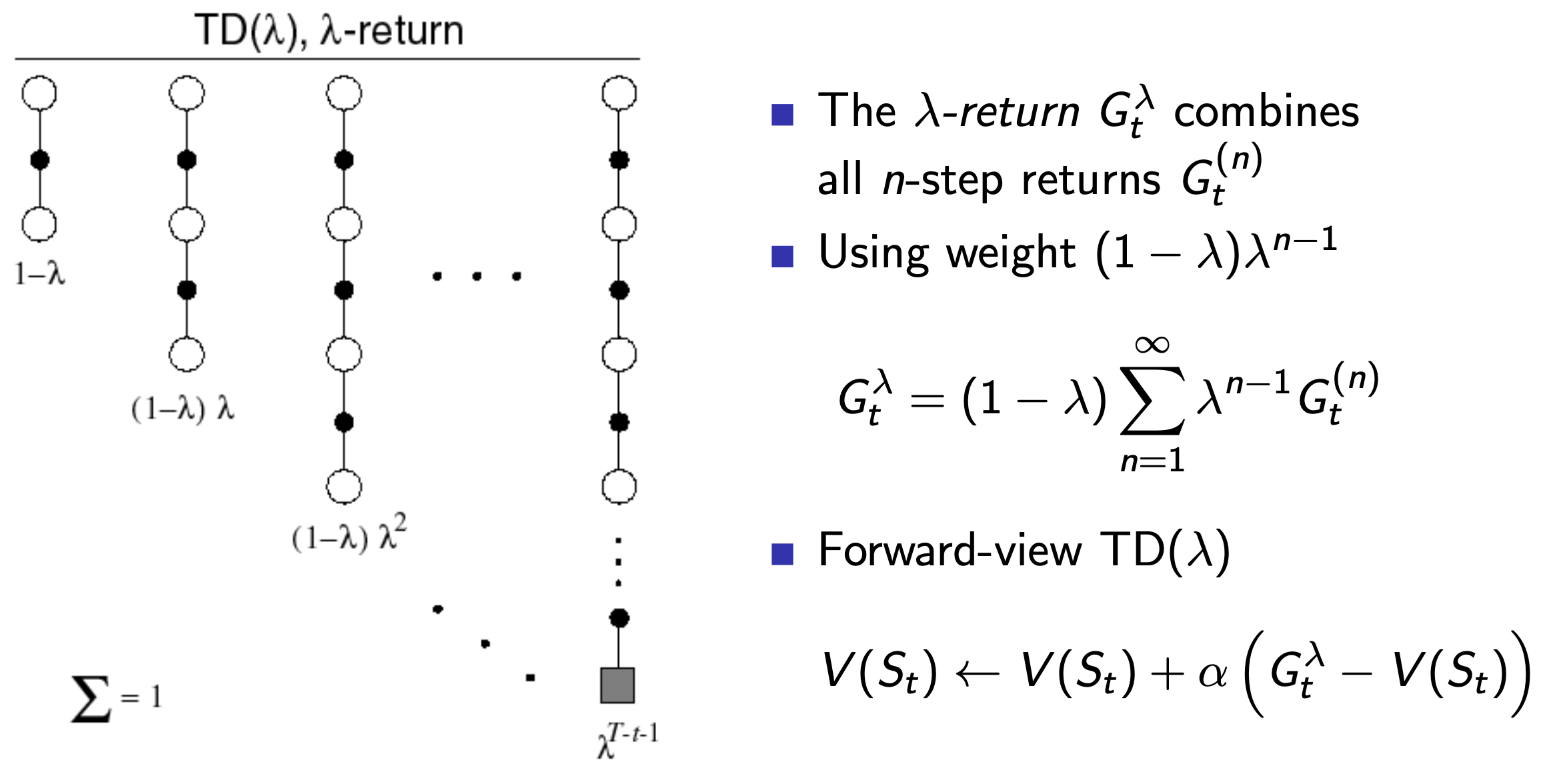

Backward View \(TD(\lambda)\)

The problem with the update rule(s) we've been using so far are that the are forward looking, and in the \(TD(\lambda)\) case this means we have to wait for the end of the episode (\(n\)-steps in the future) like in MC learning since we are using the forward view method.

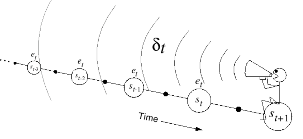
Instead we can use the backward view method where we move forwards, but at each time step \(t\), the TD error \(\delta_t\) immediately updates all previously visited states. This eliminates the need to wait for future information, each step's learning propagates backward through the episode history.

Eligibility Traces

The problem with that is the credit assignment problem: what thing that happened in the past deserves credit for success or failure? The frequency heuristic assigns credit to most frequency states, and the recency heuristic assigns credit to most recent states. Eligibility traces combine both heuristics.

Algorithm

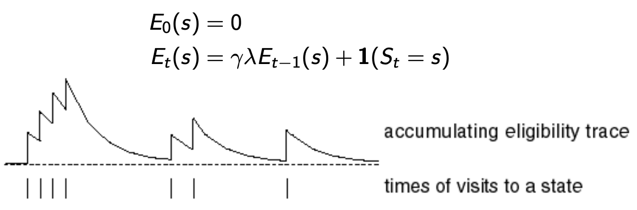
• Keep an eligibility trace for each state \(s\)

• Update value \(V(s)\) for every state \(s\) in proportion to the TD error \(\delta_t\) and the eligibility trace for that state \(E_t(s)\) \[\delta_t = (R_{t+1} +\gamma V(S_{t+1})-V_{old}(S_t)\] \[V_{new}(s) \leftarrow V_{old}(s) + \alpha \delta_t E_t(s)\]

• In this algorithm, for each new state we see, compute the TD error, and broadcast an update to any/all previous eligible states

• When \(\lambda = 0\), only the current state is updated since then \(E_t(s) = 1(S_t = s)\), which is equivalent to the default \(TD(0)\) update

• When \(\lambda = 1\), all states get a decent amount of eligibility which keeps them eligible for longer which acts to update many states when the final reward arrives, which is equivalent to the total update for MC so TD(1) = MC