Model-free Control

Sticking within the model-free setting where the reward and transition probability functions are unknown, we now discuss control. As a reminder, the control problem is to find an optimal policy \(\pi^*\) that maximizes cumulative future return.

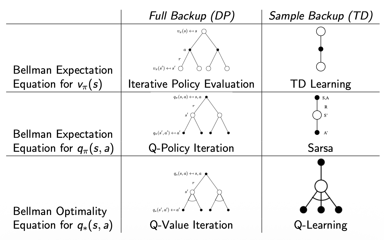
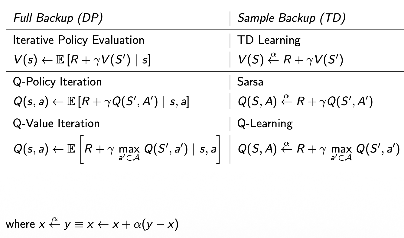
In model-free prediction we covered how to find state-value functions \(v_{\pi}\), but without a model of the environment, we don't know which actions will take us to what state. In these scenarios estimating the state-value function \(v_{\pi}(s)\) isn't useful in building an optimal policy because we can't know which action to take to get to the state with the highest value. Instead, we need to estimate the action-value function \(q_{\pi}(s,a)\), which tells us the value of taking action \(a\) from state \(s\), without needing to know where we end up. Then we can build the optimal policy by picking the action with the highest q-value. \[\pi'(s) = \text{argmax}_{a} Q(s,a)\] So in this section we will always:

1. Use some sort of policy evaluation to find the \(Q(s,a)\), typically the MC and TD methods from [[5 Model-free Prediction]]
2. Apply some sort of policy improvement to improve \(\pi\) based on \(Q(s,a)\) (this is the control part)

\(\epsilon\)-Greedy Exploration

During policy improvement, if we always improve the policy based on greedily picking the best action according to \(Q(s,a)\) then we may miss a very valuable state/action that required some exploration. In order to ensure some continual exploration we can improve the policy as such: \[\pi(a|s) = \begin{cases} \frac{\epsilon}{m} + (1 - \epsilon) & \text{if } a^* = \arg\max\limits_{a \in \mathcal{A}} Q(s, a) \\ \frac{\epsilon}{m} & \text{otherwise} \end{cases}\] where \(m\) = number of actions. So with probability \(1-\epsilon\) choose the greedy action, and with probability \(\epsilon\) choose an action at random.

Greedy in the Limit with Infinite Exploration (GLIE)

Doing a slight bit of exploration often isn't very meaningful, we're probably still missing a lot, so we introduce this GLIE property that says:

• All state-action pairs are explored infinitely many times in the limit
• The policy converges on a greedy policy in the limit

And we make \(\epsilon\)-greedy GLIE if \(\epsilon\) reduces to zero at \(\epsilon_k = \frac{1}{k}\), essentially this means we put \(\epsilon\) on a decay schedule inversely proportional with the number of episodes. We will take this as a given, the proof is out of scope.

Monte-Carlo Control

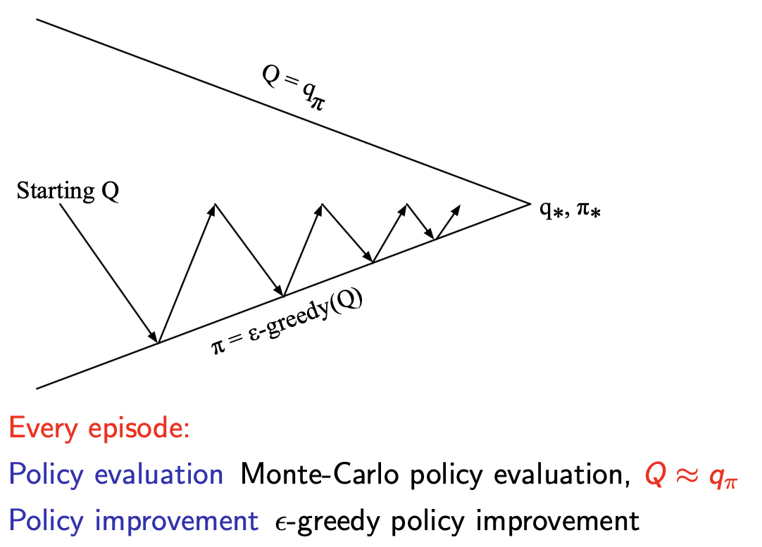
When doing control with dynamic programming we used Policy Iteration, in which we evaluated a policy in full before improving the policy. Instead, in Monte-Carlo Control, we will simply evaluate the policy for one sample episode, then improve the policy based on the new action-value function, rather than evaluating the policy until it converges. Visually it looks like partially evaluating the policy each step, but fully improving the policy each step:

Algorithm

• Sample \(k\)-th episode using \(\pi: \{S_1, A_1, R_2, \ldots, S_T\} \sim \pi\)
• For each state \(S_t\) and action \(A_t\) in the episode,
  • \(N(S_t, A_t) \leftarrow N(S_t, A_t) + 1\)
  • \(Q(S_t, A_t) \leftarrow Q(S_t, A_t) + \frac{1}{N(S_t, A_t)}(G_t - Q(S_t, A_t))\)
• Improve the policy based on new action-value function
  • \(\epsilon = 1/k\)
  • \(\pi \rightarrow \epsilon\text{greedy}(Q)\)

SARSA

Since Temporal-Difference (TD) learning has several advantages over Monte-Carlo (MC), as we saw in the previous chapter:

• Lower variance
• Online
• Incomplete sequences

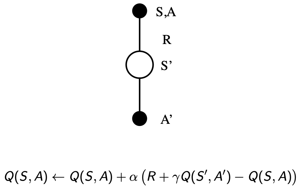
The natural idea would be to use TD instead of MC in our control loop. This method is called State-Action-Reward-State-Action (SARSA), because we start with \(S\), then take action \(A\) using policy derived from \(Q\) (e.g. \(\epsilon\)-greedy), observe reward \(R\) and state \(S'\), then choose \(A'\) from \(Q\) to get:

Forward View SARSA\((\lambda)\)

Similarly to \(TD(\lambda)\) in [[5 Model-free Prediction]], we can apply a weight over all possible \(n\)-step look-aheads and combine the return:

Backward View SARSA\((\lambda)\)

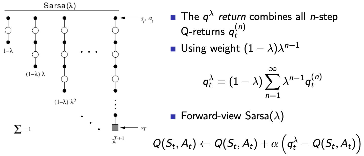
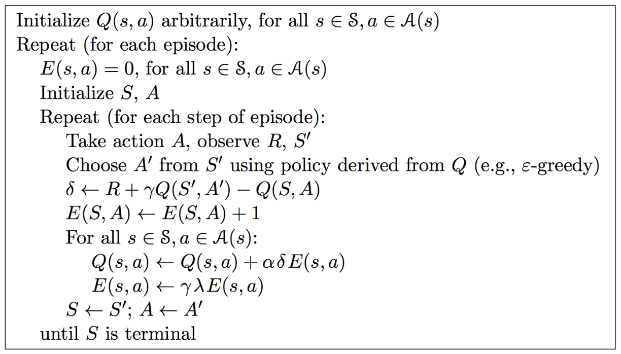
Just like \(TD(\lambda)\), we can use eligibility traces to make this an online algorithm:

• \(E_{0}(s,a) = 0\)

• \(E_t(s,a) = \gamma \lambda E_{t-1}(s,a) + 1(S_t = s, A_t = a)\) \(Q(s,a)\) is updated for every state \(s\) and action \(a\), in proportion to TD-error \(\delta_t\) and eligibility trace \(E_t(s,a)\)

• \(\delta_t = (R_{t+1} + \gamma Q(S_{t+1}, A_{t+1})) - Q(S_t, A_t)\)

• \(Q(s,a) \leftarrow Q(s,a) + \alpha \delta_t E_t(s,a)\)

  

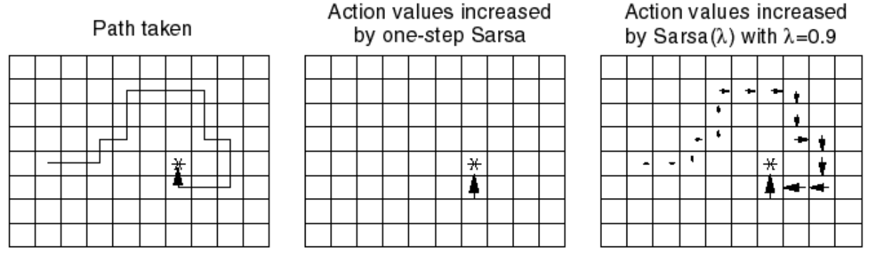
The value and beauty of SARSA\((\lambda)\) becomes evident when you see examples like the following, where it enables all state-action pairs that contributed to the reward at the end to accumulate proportional reward:

Off-Policy Learning

In cases where we want to do any of the following, we must use Off-Policy Learning:

• Learn from observing humans or other agents
• Re-use experience generated from old policies
• Learn about optimal policy while following an exploratory policy
• Learn about multiply policies while following one policy

This is because, let's say we want to be more exploratory in training, if we use a high \(\epsilon\)-greedy policy improvement then the target policy itself will become exploratory. Since in the Q-function update rules we use \(A'\) by sampling from the \(\epsilon\)-greedy policy, the learned Q-values represent expected returns under the \(\epsilon\)-greedy policy, that is, the optimal actions under this learned value function still assume future randomness in proportion to \(\epsilon\). So in this scenario if we learn using an exploratory policy we cannot turn that off when it is time to use that policy in reality.

Q-Learning

If we want to do off-policy prediction, or learning of action-values \(Q(s,a)\):

• The action is chosen using the behaviour policy \(A_t \sim \mu(\cdot|S_t)\)
• The successor action is chosen from our target policy \(A' \sim \pi(\cdot|S_t)\) The update rule becomes: \[Q(S_t, A_t) \leftarrow Q(S_t, A_t) + \alpha (\textcolor{red}{R_{t+1} + \gamma Q(S_{t+1}, A'}) - Q(S_t, A_t))\] So here we are updating the Q-values for our target policy \(\pi\) by rolling out \(\mu\) for immediate action \(A_t\), and then computing the error based on \(A'\) an action from \(\pi\). This allows us to explore using \(\mu\), but use \(A'\) from \(\pi\) in the error calculation to learn \(Q_{\pi}(s,a)\) rather than \(Q_{\mu}(s,a)\). If we used another action from \(\mu\) we'd learn about the exploratory policy instead of our target.

We want to learn \(Q_{\pi}(s,a)\) for all state-action pairs, but our target policy \(\pi\) (being greedy) would never take suboptimal actions. The behavior policy \(\mu\) lets us experience those actions, then we evaluate them assuming we follow \(\pi\) thereafter.

Example: If \(\mu\) takes "attack" in "low health" state, we learn \(Q_{\pi}(\text{low health, attack})\) by observing the immediate result, then assuming \(\pi\) (which would choose "heal" for the next action) for all future steps. This gives us the value of "attack" under policy \(\pi\) without forcing \(\pi\) to actually take that suboptimal action.

Off-Policy Control

We now allow both behaviour and target policies to improve:

• The target policy \(\pi\) is greedy w.r.t. \(Q(s,a)\): it always chooses the action with highest Q-value
• The behaviour policy \(\mu\) is exploratory (e.g. \(\epsilon\)-greedy w.r.t \(Q(s,a)\))

Since \(\pi\) is greedy, when we need to choose \(A' \sim \pi(\cdot|S_{t+1})\) for our target calculation, we get: \[A' = \text{argmax}_{a'} Q(S_{t+1}, a')\] This means the Q-learning target simplifies from: \[R_{t+1} + \gamma Q(S_{t+1}, A')\] to: \[R_{t+1} + \gamma Q(S_{t+1}, \text{argmax}_{a'} Q(S_{t+1}, a')) = R_{t+1} + \gamma \max_{a'} Q(S_{t+1}, a')\] The beauty is that \(\mu\) can explore suboptimal actions (letting us learn about them), while our target calculation always assumes we'll act optimally going forward (using the max over actions).

Q-Learning Control Algorithm

\[Q(S, A) \leftarrow Q(S,A) + \alpha (R + \gamma \text{max}_{a'}Q(S',a') - Q(S,A))\]

Relationship Between DP and TD