An Analytical Approach to Batch Normalization Gradients

In this note I want to share a method of computing an analytical gradient for Batch Normalization that I found to be most clear and understandable, to me.

I was prompted to do this while working on assignment 2 from CS231n, where you are asked to derive and implement the backward pass for batch normalization from scratch. To my understanding there are two ways to do this:

1. Computational graph: break the function into it's individual operations, compute the local derivatives, and multiply them using the chain rule
2. Analytical derivative: write out the function, take it's derivative with respect to it's inputs

I tried to take the analytical derivative approach because I found that it made the process most intuitive, given that you understand the chain rule. There are a few other blog posts on this topic, one uses the computational graph approach, two and three use the analytical gradient derivative. This note will aim to be more explanatory in both the maths and the code. We will assume you understand BatchNorm, Calculus 1 derivative rules, and the conceptual different between a derivative and a partial derivative.

Some advice in reading this: it takes some time to load the priors of Batch Norm into your head, so skipping parts or scrolling through the note will probably confuse you and serve as discouragement. You will get the most out of this by following along from the beginning and writing down your understanding as you go, stopping if you get confused to rectify that confusion, and repeating.

Finally, I'm aware that BatchNorm isn't really used in practice very much anymore, in favour of alternatives such as LayerNorm and GroupNorm, but I believe deriving and implementing the backward pass for BatchNorm is a valuable exercise for newcomers to deep learning because the input effects the output in several different ways, making for a complicated practice problem.

Please write to me with any feedback, errata, or thoughts via email or X.

Chain Rule Primer

Before diving into the batch normalization gradient derivation, let's review the multivariable chain rule since it's the foundation of our approach.

Consider a function \(u(x,y)\) where both \(x\) and \(y\) are themselves functions of other variables, say \(x(r,t)\) and \(y(r,t)\). When we want to find how \(u\) changes with respect to \(r\), we need to account for all the ways that \(r\) influences \(u\). Since \(r\) affects \(u\) through both \(x\) and \(y\), the chain rule tells us: \[\frac{\partial u}{\partial r} = \frac{\partial u}{\partial x} \cdot \frac{\partial x}{\partial r} + \frac{\partial u}{\partial y} \cdot \frac{\partial y}{\partial r}\] This principle extends naturally to functions with more variables. The key insight is that we sum up all the "pathways" through which our variable of interest can influence the final output. In batch normalization, this becomes particularly important because the input affects the output through multiple computational paths.

Notation

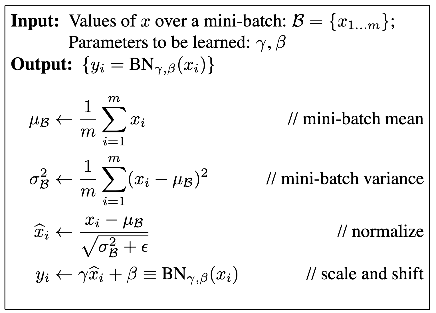
From the original paper BatchNorm is given as: We will use the same notation, and additionally use \(f\) to refer to the layer after the BN layer.

Gradient Derivation

Gradient with respect to the input

We start by deriving the gradient of \(f\) with respect to the a single input \(x_i\). Using the chain rule, we have:

\[\frac{df}{dx_i} = \sum_j \left( \frac{\partial f}{\partial y_j} \cdot \frac{\partial y_j}{\partial x_i} \right)\] where:

• \(\frac{\partial f}{\partial y_j}\) is the effect of a single \(y_j\) on \(f\), and
• \(\frac{\partial y_j}{\partial x_i}\) is the effect of a single \(x_i\) on a single \(y_j\)

You may be confused by the summation, but the reason for it is that a single input \(x_i\) affects every single output \(y_j\) in the batch, not just \(y_i\). This happens because batch normalization uses shared statistics (mean and variance) computed across the entire batch. More specifically, \(x_i\) influences each \(y_j\) through three distinct pathways:

1. Direct path: \(x_i\) directly affects \(\hat{x}_i\) (only when \(i = j\))
2. Mean path: \(x_i\) contributes to \(\mu_B\), which is used to normalize all \(\hat{x}_j\)
3. Variance path: \(x_i\) contributes to \(\sigma_B^2\), which is used to normalize all \(\hat{x}_j\)

Since we want to find how \(f\) changes with respect to \(x_i\), we need to sum up \(x_i\)'s influence on all the outputs \(y_j\) that contribute to \(f\). This is exactly what the summation \(\sum_j\) captures.

Now let's break down the effect of a single input \(x_i\) on a single output \(y_j\) \((\frac{\partial y_j}{\partial x_i})\) using the very same method from the chain rule refresher above: \[\frac{\partial y_j}{\partial x_i} = \underbrace{\textcolor{green}{\frac{\partial y_j}{\partial \hat{x}_j} \cdot \frac{\partial \hat{x}_j}{\partial x_i}}}_{\text{direct path}} + \underbrace{\textcolor{blue}{\frac{\partial y_j}{\partial \hat{x}_j} \cdot \frac{\partial \hat{x}_j}{\partial \mu_B}} \cdot \textcolor{blue}{\frac{\partial \mu_B}{\partial x_i}}}_{\text{mean path}} + \underbrace{\textcolor{red}{\frac{\partial y_j}{\partial \hat{x}_j} \cdot \frac{\partial \hat{x}_j}{\partial \sigma_B^2}} \cdot \textcolor{red}{\frac{\mathrm{d} \sigma_B^2}{\mathrm{d} x_i}}}_{\text{variance path}}\] Factoring out \(\frac{\partial y_j}{\partial \hat{x}_j}\) we get: \[\frac{\partial y_j}{\partial x_i} = \frac{\partial y_j}{\partial \hat{x}_j} \left( \underbrace{\textcolor{green}{\frac{\partial \hat{x}_j}{\partial x_i}}}_{\text{direct}} + \underbrace{\textcolor{blue}{\frac{\partial \hat{x}_j}{\partial \mu_B} \cdot \frac{\partial \mu_B}{\partial x_i}}}_{\text{mean}} + \underbrace{\textcolor{red}{\frac{\partial \hat{x}_j}{\partial \sigma_B^2} \cdot \frac{\mathrm{d} \sigma_B^2}{\mathrm{d} x_i}}}_{\text{variance}} \right)\]

Now let's compute each pathway step by step.

Direct Path

For the direct path, we need to compute \(\textcolor{green}{\frac{\partial \hat{x}_j}{\partial x_i}}\). Recall that \(\hat{x}_j = \frac{x_j - \mu_B}{\sqrt{\sigma_B^2 + \epsilon}}\). When we take the partial derivative with respect to \(x_i\), we only get a non-zero result when \(j = i\) (since \(x_j\) doesn't directly depend on \(x_i\) unless they're the same variable).

\[\textcolor{green}{\frac{\partial \hat{x}_j}{\partial x_i}} = \begin{cases} \frac{1}{\sqrt{\sigma_B^2 + \epsilon}} & \text{if } i = j \\ 0 & \text{if } i \neq j \end{cases}\]

This can be written compactly using the Kronecker delta \(\delta_{ij}\), which equals 1 when \(i = j\) and 0 otherwise:

\[\textcolor{green}{\frac{\partial \hat{x}_j}{\partial x_i}} = \frac{\delta_{ij}}{\sqrt{\sigma_B^2 + \epsilon}}\]

Mean Path

For the mean path, we need two derivatives: \(\textcolor{blue}{\frac{\partial \hat{x}_j}{\partial \mu_B}}\) and \(\textcolor{blue}{\frac{\partial \mu_B}{\partial x_i}}\). First, \(\textcolor{blue}{\frac{\partial \hat{x}_j}{\partial \mu_B}}\): \[\hat{x}_j = \frac{x_j - \mu_B}{\sqrt{\sigma_B^2 + \epsilon}}\] When taking the partial derivative with respect to \(\mu_B\), both \(x_j\) and \(\sqrt{\sigma_B^2 + \epsilon}\) are treated as constants. We're essentially differentiating \((x_j - \mu_B)\) with respect to \(\mu_B\), which gives us \(-1\), then multiplying by the constant coefficient \(\frac{1}{\sqrt{\sigma_B^2 + \epsilon}}\):

\[\textcolor{blue}{\frac{\partial \hat{x}_j}{\partial \mu_B}} = \frac{-1}{\sqrt{\sigma_B^2 + \epsilon}}\] Next, \(\textcolor{blue}{\frac{\partial \mu_B}{\partial x_i}}\): \[\mu_B = \frac{1}{N} \sum_{k=1}^N x_k = \frac{1}{N}(x_1 + x_2 + \cdots + x_i + \cdots + x_N)\]

When we expand the summation and take the partial derivative with respect to \(x_i\), all terms \(x_k\) where \(k \neq i\) are constants and disappear. Only the \(x_i\) term remains, which has derivative \(1\), leaving us with the coefficient: \[\textcolor{blue}{\frac{\partial \mu_B}{\partial x_i}} = \frac{1}{N}\]

Variance Path

For the variance path, we need two derivatives: \(\textcolor{red}{\frac{\partial \hat{x}_j}{\partial \sigma_B^2}}\) and \(\textcolor{red}{\frac{\partial \sigma_B^2}{\partial x_i}}\).

First, \(\textcolor{red}{\frac{\partial \hat{x}_j}{\partial \sigma_B^2}}\): \[\hat{x}_j = (x_j - \mu_B)(\sigma_B^2 + \epsilon)^{-1/2}\]

When taking the partial derivative with respect to \(\sigma_B^2\), the term \((x_j - \mu_B)\) is treated as a constant coefficient. We're differentiating \((\sigma_B^2 + \epsilon)^{-1/2}\) with respect to \(\sigma_B^2\) using the power rule: the exponent \(-1/2\) becomes the coefficient, and we subtract 1 from the exponent to get \(-3/2\):

\[\textcolor{red}{\frac{\partial \hat{x}_j}{\partial \sigma_B^2}} = (x_j - \mu_B) \cdot \left(-\frac{1}{2}\right)(\sigma_B^2 + \epsilon)^{-3/2} = -\frac{(x_j - \mu_B)}{2(\sigma_B^2 + \epsilon)^{3/2}}\] Next, \(\textcolor{red}{\frac{d \sigma_B^2}{d x_i}}\):

This requires a total derivative (not a partial derivative) because \(\sigma_B^2\) depends on \(x_i\) in two ways: directly through the \(x_i\) term when \(k=i\) in the summation, and indirectly through \(\mu_B\) (since \(\mu_B\) itself depends on all \(x_k\) including \(x_i\)). The other derivatives we computed earlier were partial derivatives because they only had one pathway of dependence. \[\sigma_B^2 = \frac{1}{N} \sum_{k=1}^N (x_k - \mu_B)^2\] Using the chain rule for total derivatives: \[\textcolor{red}{\frac{d \sigma_B^2}{d x_i}} = \frac{\partial \sigma_B^2}{\partial x_i} + \frac{\partial \sigma_B^2}{\partial \mu_B} \cdot \frac{\partial \mu_B}{\partial x_i}\]

For the first term \(\frac{\partial \sigma_B^2}{\partial x_i}\): when we treat \(\mu_B\) as constant and differentiate \((x_i - \mu_B)^2\) with respect to \(x_i\), we get \(2(x_i - \mu_B)\), multiplied by the coefficient \(\frac{1}{N}\): \[\frac{\partial \sigma_B^2}{\partial x_i} = \frac{2(x_i - \mu_B)}{N}\]

For the second term \(\frac{\partial \sigma_B^2}{\partial \mu_B}\): when we treat all \(x_k\) as constants and differentiate each \((x_k - \mu_B)^2\) with respect to \(\mu_B\), we get \(-2(x_k - \mu_B)\) for each term: \[\frac{\partial \sigma_B^2}{\partial \mu_B} = \frac{1}{N} \sum_{k=1}^N -2(x_k - \mu_B) = \frac{-2}{N} \sum_{k=1}^N (x_k - \mu_B)\]

Expanding the summation: \[\frac{\partial \sigma_B^2}{\partial \mu_B} = \frac{-2}{N} \left( \sum_{k=1}^N x_k - \sum_{k=1}^N \mu_B \right) = \frac{-2}{N} \left( \sum_{k=1}^N x_k - N\mu_B \right)\]

Since \(\mu_B = \frac{1}{N} \sum_{k=1}^N x_k\), we have \(\sum_{k=1}^N x_k = N\mu_B\), so: \[\frac{\partial \sigma_B^2}{\partial \mu_B} = \frac{-2}{N}(N\mu_B - N\mu_B) = \frac{-2}{N} \cdot 0 = 0\]

Therefore, the second term vanishes entirely, and we get: \[\textcolor{red}{\frac{d \sigma_B^2}{d x_i}} = \frac{2(x_i - \mu_B)}{N}\]

Combining the paths

Now let's combine all the paths. Recall our original expression: \[\frac{\partial y_j}{\partial x_i} = \frac{\partial y_j}{\partial \hat{x}_j} \left( \underbrace{\textcolor{green}{\frac{\partial \hat{x}_j}{\partial x_i}}}_{\text{direct}} + \underbrace{\textcolor{blue}{\frac{\partial \hat{x}_j}{\partial \mu_B} \cdot \frac{\partial \mu_B}{\partial x_i}}}_{\text{mean}} + \underbrace{\textcolor{red}{\frac{\partial \hat{x}_j}{\partial \sigma_B^2} \cdot \frac{\mathrm{d} \sigma_B^2}{\mathrm{d} x_i}}}_{\text{variance}} \right)\]

From our calculations above, we found:

• Direct path: \(\textcolor{green}{\frac{\partial \hat{x}_j}{\partial x_i}} = \frac{\delta_{ij}}{\sqrt{\sigma_B^2 + \epsilon}}\)
• Mean path: \(\textcolor{blue}{\frac{\partial \hat{x}_j}{\partial \mu_B} \cdot \frac{\partial \mu_B}{\partial x_i}} = \frac{-1}{\sqrt{\sigma_B^2 + \epsilon}} \cdot \frac{1}{N} = \frac{-1}{N\sqrt{\sigma_B^2 + \epsilon}}\)
• Variance path: \(\textcolor{red}{\frac{\partial \hat{x}_j}{\partial \sigma_B^2} \cdot \frac{\mathrm{d} \sigma_B^2}{\mathrm{d} x_i}} = \frac{-(x_j - \mu_B)}{2(\sigma_B^2 + \epsilon)^{3/2}} \cdot \frac{2(x_i - \mu_B)}{N} = \frac{-(x_j - \mu_B)(x_i - \mu_B)}{N(\sigma_B^2 + \epsilon)^{3/2}}\)

We also need \(\frac{\partial y_j}{\partial \hat{x}_j}\). Since \(y_j = \gamma \hat{x}_j + \beta\): \[\frac{\partial y_j}{\partial \hat{x}_j} = \gamma\] Substituting everything into our original expression: \[\frac{\partial y_j}{\partial x_i} = \gamma \left( \textcolor{green}{\frac{\delta_{ij}}{\sqrt{\sigma_B^2 + \epsilon}}} - \textcolor{blue}{\frac{1}{N\sqrt{\sigma_B^2 + \epsilon}}} - \textcolor{red}{\frac{(x_j - \mu_B)(x_i - \mu_B)}{N(\sigma_B^2 + \epsilon)^{3/2}}} \right)\]

We could factor out the inverse variance and make this cleaner, and thereby also make our code later cleaner, but I prefer to leave it this way because it's most intuitive to understand. This expression captures how each input \(x_i\) influences each output \(y_j\) through all three pathways we identified.

Complete gradient with respect to the input

Now we can substitute our result back into the original expression to get the complete gradient of \(f\) with respect to \(x_i\): \[\frac{df}{dx_i} = \sum_j \left( \frac{\partial f}{\partial y_j} \cdot \frac{\partial y_j}{\partial x_i} \right)\] Substituting our expression for \(\frac{\partial y_j}{\partial x_i}\):

\[\frac{df}{dx_i} = \sum_j \frac{\partial f}{\partial y_j} \cdot \gamma \left( \textcolor{green}{\frac{\delta_{ij}}{\sqrt{\sigma_B^2 + \epsilon}}} - \textcolor{blue}{\frac{1}{N\sqrt{\sigma_B^2 + \epsilon}}} - \textcolor{red}{\frac{(x_j - \mu_B)(x_i - \mu_B)}{N(\sigma_B^2 + \epsilon)^{3/2}}} \right)\]

Factoring out \(\gamma\) and distributing the summation:

\[\frac{df}{dx_i} = \gamma \left[ \textcolor{green}{\sum_j \frac{\partial f}{\partial y_j} \frac{\delta_{ij}}{\sqrt{\sigma_B^2 + \epsilon}}} - \textcolor{blue}{\sum_j \frac{\partial f}{\partial y_j} \frac{1}{N\sqrt{\sigma_B^2 + \epsilon}}} - \textcolor{red}{\sum_j \frac{\partial f}{\partial y_j} \frac{(x_j - \mu_B)(x_i - \mu_B)}{N(\sigma_B^2 + \epsilon)^{3/2}}} \right]\]

Now we can simplify each colored term:

• Direct path: The Kronecker delta \(\delta_{ij}\) means only the \(j=i\) term survives
• Mean path: Constants can be factored out of the summation
• Variance path: The \((x_i - \mu_B)\) term can be factored out

\[\frac{df}{dx_i} = \gamma \left[ \textcolor{green}{\frac{\partial f}{\partial y_i} \frac{1}{\sqrt{\sigma_B^2 + \epsilon}}} - \textcolor{blue}{\frac{1}{N\sqrt{\sigma_B^2 + \epsilon}} \sum_j \frac{\partial f}{\partial y_j}} - \textcolor{red}{\frac{(x_i - \mu_B)}{N(\sigma_B^2 + \epsilon)^{3/2}} \sum_j \frac{\partial f}{\partial y_j} (x_j - \mu_B)} \right]\]

This is our final expression for the gradient with respect to the input \(x_i\). Notice how the three pathways are still clearly visible:

• Direct: Only affects the gradient through \(\frac{\partial f}{\partial y_i}\) (the output at the same index)
• Mean: Affects the gradient through the sum of all upstream gradients \(\sum_j \frac{\partial f}{\partial y_j}\)
• Variance: Affects the gradient through a weighted sum where each upstream gradient is weighted by how far that output's input was from the mean

That concludes the derivations for the gradient with respect to the input \(x_i\). If you got lost along the way somewhere, email me, and I'll try to help. I'd also like to hear from you if you found the explanation intuitive, I found other explanations difficult to grasp owing to my shortcomings in maths, but this worked well for me!

Gradient with respect to gamma

Next we need to find the effect of the scale parameter \(\gamma\) on \(f\), i.e. find \(\frac{df}{d\gamma}\). Again we use the chain rule. Since \(\gamma\) affects all outputs \(y_i\) in the batch, we need to sum the effect \(\gamma\) had on all \(y_i\): \[\frac{df}{d\gamma} = \sum_i \frac{\partial f}{\partial y_i} \cdot \frac{\partial y_i}{\partial \gamma}\]

We need \(\frac{\partial y_i}{\partial \gamma}\). Recall that \(y_i = \gamma \hat{x}_i + \beta\): When taking the partial derivative with respect to \(\gamma\), the term \(\beta\) disappears (it's a constant), and \(\hat{x}_i\) becomes the coefficient: \[\frac{\partial y_i}{\partial \gamma} = \hat{x}_i\] Therefore: \[\frac{df}{d\gamma} = \sum_i \frac{\partial f}{\partial y_i} \cdot \hat{x}_i\]

Gradient with respect to beta

Similarly, for \(\frac{df}{d\beta}\): \[\frac{df}{d\beta} = \sum_i \frac{\partial f}{\partial y_i} \cdot \frac{\partial y_i}{\partial \beta}\]

We need \(\frac{\partial y_i}{\partial \beta}\). From \(y_i = \gamma \hat{x}_i + \beta\): When taking the partial derivative with respect to \(\beta\), the term \(\gamma \hat{x}_i\) disappears (it's treated as a constant), leaving us with: \[\frac{\partial y_i}{\partial \beta} = 1\] Therefore: \[\frac{df}{d\beta} = \sum_i \frac{\partial f}{\partial y_i} \cdot 1 = \sum_i \frac{\partial f}{\partial y_i}\]

These gradients are much more straightforward than the input gradient because \(\gamma\) and \(\beta\) directly scale and shift the normalized values without the complex interdependencies we saw with the shared batch statistics.

Implementation

Now that we've derived the mathematical expressions for all gradients, let's see how to implement them efficiently using vectorized NumPy operations. The key challenge is understanding how the mathematical summations and individual terms map to vectorized array operations.

Here's our final vectorized implementation for reference:

def batchnorm_backward(dout, cache):
    # dout: (N, D) - upstream gradients 
    # returns: dx (N, D), dgamma (D,), dbeta (D,)
    (mean, inv_var, x, x_hat, gamma) = cache
    N, D = x_hat.shape
    
    # Gradients for learnable parameters
    dgamma = np.sum(dout * x_hat, axis=0)
    dbeta = np.sum(dout, axis=0)
    
    # Input gradient: three pathway terms
    # Direct contribution from x_i
    term1 = dout * gamma * inv_var
    
    # Contribution from mean (mu)
    term2 = -gamma * (1. / N) * inv_var * np.sum(dout, axis=0)
    
    # Contribution from variance (sigma^2)
    term3 = -gamma * (1. / N) * (x-mean) * inv_var**3 * np.sum(dout * (x - mean), axis=0)
    
    dx = term1 + term2 + term3
    
    return dx, dgamma, dbeta

We'll break down how each mathematical expression maps to vectorized code.

Input Gradient: Term 1 (Direct Path)

\[\frac{df}{dx_i} = \textcolor{green}{\frac{\partial f}{\partial y_i} \frac{\gamma}{\sqrt{\sigma_B^2 + \epsilon}}} - \frac{\gamma}{N\sqrt{\sigma_B^2 + \epsilon}} \sum_j \frac{\partial f}{\partial y_j} - \frac{\gamma(x_i - \mu_B)}{N(\sigma_B^2 + \epsilon)^{3/2}} \sum_j \frac{\partial f}{\partial y_j} (x_j - \mu_B)\]

The green expression above representing the direct path becomes the following code:

term1 = dout * gamma * inv_var

This is the direct pathway where \(x_i\) only affects \(y_i\) (not other outputs). The Kronecker delta \(\delta_{ij}\) from our derivation automatically becomes element-wise multiplication in the vectorized implementation:

• dout[i] (\(i\)-th row) contains \(\frac{\partial f}{\partial y_i}\) (upstream gradient for output \(i\))
• gamma contains \(\gamma\) (scale parameter)
• inv_var contains \(\frac{1}{\sqrt{\sigma_B^2 + \epsilon}}\) (inverse standard deviation)
• Since this is an element-wise multiplication, it naturally pairs each term1[i] with its corresponding dout[i]
  • term1[0] gets dout[0] * gamma * inv_var = \(\frac{\partial f}{\partial y_0} \frac{\gamma}{\sqrt{\sigma_B^2 + \epsilon}}\)
  • term1[1] gets dout[1] * gamma * inv_var = \(\frac{\partial f}{\partial y_1} \frac{\gamma}{\sqrt{\sigma_B^2 + \epsilon}}\)
  • term1[2] gets dout[2] * gamma * inv_var = \(\frac{\partial f}{\partial y_2} \frac{\gamma}{\sqrt{\sigma_B^2 + \epsilon}}\)

Input Gradient: Term 2 (Mean Path)

\[\frac{df}{dx_i} = \frac{\partial f}{\partial y_i} \frac{\gamma}{\sqrt{\sigma_B^2 + \epsilon}} \textcolor{blue}{ - \frac{\gamma}{N\sqrt{\sigma_B^2 + \epsilon}} \sum_j \frac{\partial f}{\partial y_j}} - \frac{\gamma(x_i - \mu_B)}{N(\sigma_B^2 + \epsilon)^{3/2}} \sum_j \frac{\partial f}{\partial y_j} (x_j - \mu_B)\]

The blue expression above representing the mean path becomes the following code:

term2 = -gamma * (1. / N) * inv_var * np.sum(dout, axis=0)

This captures how \(x_i\) affects all outputs through the shared mean \(\mu_B\):

• np.sum(dout, axis=0) computes \(\sum_j \frac{\partial f}{\partial y_j}\) (sum of upstream gradients across the batch). To understand this: dout has shape (N, D) where each row dout[j] contains \(\frac{\partial f}{\partial y_j}\). When we sum along axis=0, we're adding up all the rows: dout[0] + dout[1] + ... + dout[N-1], which gives us exactly \(\sum_j \frac{\partial f}{\partial y_j}\) for each feature dimension.
• The result has shape (D,), because np.sum will collapse the columns of the (N,D) array, leaving one value per feature dimension
• The rest of the multiplications are straight from the expression

Input Gradient: Term 3 (Variance Path)

\[\frac{df}{dx_i} = \frac{\partial f}{\partial y_i} \frac{\gamma}{\sqrt{\sigma_B^2 + \epsilon}} - \frac{\gamma}{N\sqrt{\sigma_B^2 + \epsilon}} \sum_j \frac{\partial f}{\partial y_j} \textcolor{red}{- \frac{\gamma(x_i - \mu_B)}{N(\sigma_B^2 + \epsilon)^{3/2}} \sum_j \frac{\partial f}{\partial y_j} (x_j - \mu_B)}\]

Lastly, the red expression above representing the variance path becomes:

term3 = -gamma * (1. / N) * (x-mean) * inv_var**3 * np.sum(dout * (x - mean), axis=0)

This captures how \(x_i\) affects all outputs through the shared variance \(\sigma_B^2\):

• The first (x-mean) (outside the np.sum) represents \((x_i - \mu_B)\) - the distance of each specific input from the mean. This gives us a separate value for each example in the batch.
• The second (x-mean) (inside the np.sum) represents \((x_j - \mu_B)\) when summed. Specifically, np.sum(dout * (x - mean), axis=0) computes \(\sum_j \frac{\partial f}{\partial y_j} (x_j - \mu_B)\) by summing across all examples: dout[0]*(x[0]-mean) + dout[1]*(x[1]-mean) + ... + dout[N-1]*(x[N-1]-mean).
• inv_var**3 gives us \(\frac{1}{(\sigma_B^2 + \epsilon)^{3/2}}\)
• The final multiplication combines all terms, with broadcasting automatically applying the summed result to all examples in the batch

Gamma Gradient

\[\frac{df}{d\gamma} = \sum_i \frac{\partial f}{\partial y_i} \cdot \hat{x}_i\]

becomes

dgamma = np.sum(dout * x_hat, axis=0)

This captures how each normalized input \(\hat{x}_i\) scales the effect of \(\gamma\) on the final loss:

• dout * x_hat gives us \(\frac{\partial f}{\partial y_i} \cdot \hat{x}_i\) for each example (element-wise)
• np.sum(..., axis=0) sums across the batch dimension, giving us one gradient value per feature

Beta Gradient

\[\frac{df}{d\beta} = \sum_i \frac{\partial f}{\partial y_i}\] becomes

dbeta = np.sum(dout, axis=0)

• dout contains \(\frac{\partial f}{\partial y_i}\) for each output
• np.sum(..., axis=0) sums across the batch dimension
• Since \(\beta\) simply adds a constant to each output, its gradient is just the sum of all upstream gradients

Final Remarks

If you made it this far, thank you for reading, please reach out and let me know what you thought over email or X! While I was studying this material I found that keeping all the intermediate variables and their dependencies in my head was too hard and clouded my understanding of what I'm doing. Whereas I found that using the "three pathways" framing and applying the chain rule made it much easier to keep context of where I was in the derivation and what it meant, in english. I'm curious to hear what you think.

Good luck :)

Namra